計算幾何完全指南 — 凸包、線段交點與掃描線演算法 | 資料結構與演算法
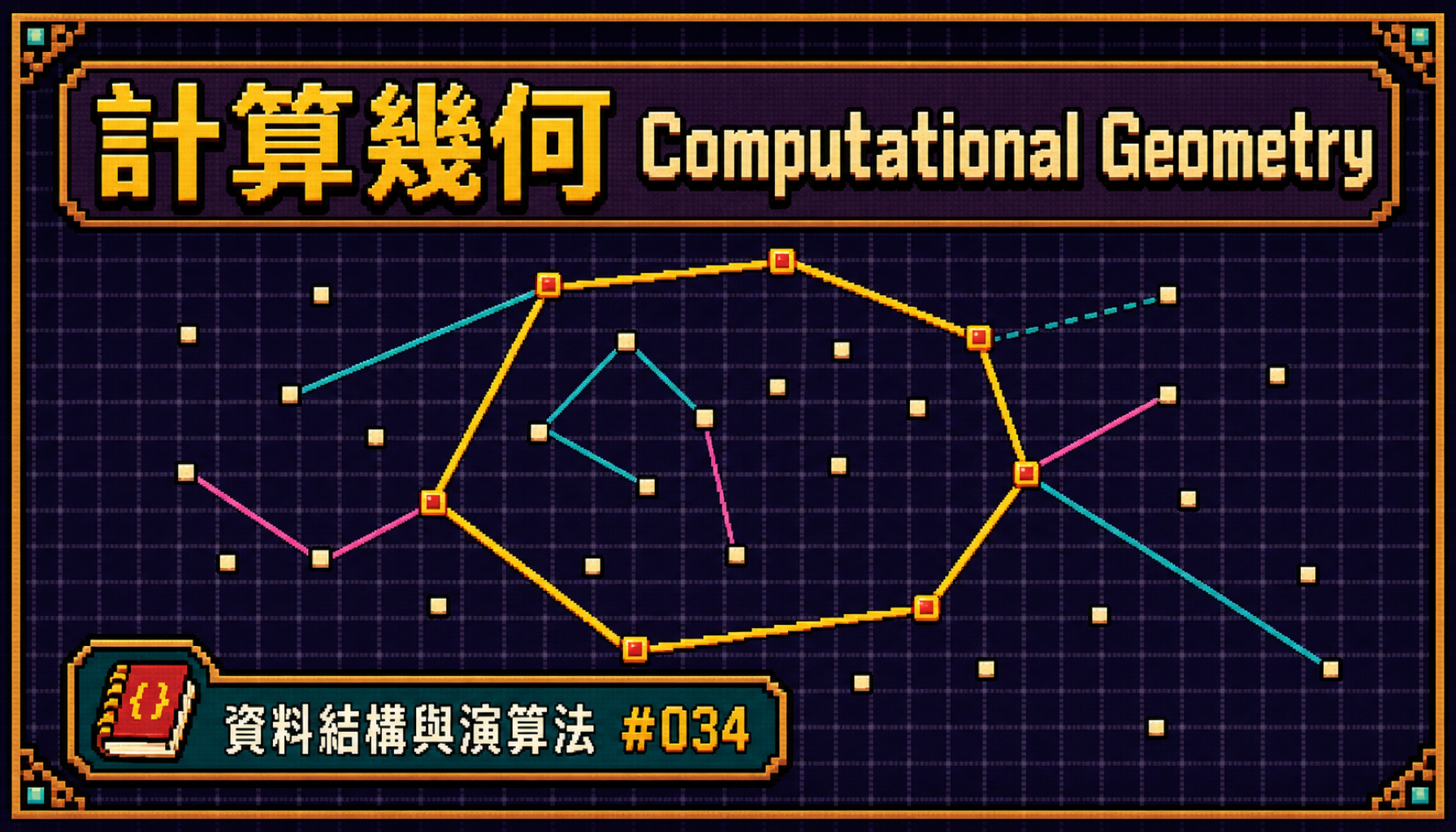
計算幾何(Computational Geometry) 是演算法中最具視覺直覺的分支,核心工具包括 叉積(Cross Product) 方向判斷、凸包(Convex Hull) 建構、線段交叉判定(Segment Intersection) 與 旋轉卡尺(Rotating Calipers)。從地圖圍欄(Geofencing)、遊戲碰撞偵測(Collision Detection),到機器人路徑規劃與 3D 列印切片,計算幾何無處不在。本文帶你從向量基礎出發,逐步掌握凸包演算法、線段交叉判定、多邊形面積計算、點在多邊形內判斷等核心技術,搭配 JavaScript/TypeScript 與 C++ 雙語言完整實作,全面解鎖計算幾何的實戰能力。
前言
想像你是一位牧場主人,手上有一把釘子散落在草地上,你想用最少的籬笆圍住所有釘子——這就是 凸包(Convex Hull) 問題。再想像你是一位城市規劃師,需要判斷兩條馬路是否交叉——這就是 線段相交判定 問題。又或者你在開發手機 App,需要判斷使用者的 GPS 座標是否在某個商圈範圍內——這就是 點在多邊形內 問題。
這些看似不同的問題,背後都共享同一套數學工具:向量運算 與 叉積。計算幾何(Computational Geometry)正是研究如何用演算法高效解決這類幾何問題的學科。
在程式設計的世界中,計算幾何的應用極為廣泛:
- 地圖服務:Geofencing 判斷使用者是否在指定區域內
- 遊戲引擎:2D/3D 碰撞偵測、視野範圍計算
- 機器人學:路徑規劃、障礙物迴避
- 電腦圖學:多邊形裁剪、光線追蹤
- 演算法競賽:凸包、掃描線、最近點對等經典題型
學習本文後,你將能夠:
- 理解 點(Point) 與 向量(Vector) 的基本運算
- 掌握 叉積(Cross Product) 的幾何意義與方向判斷
- 實作 Graham Scan 與 Andrew’s Monotone Chain 兩種凸包演算法
- 判斷 兩線段是否相交 並計算交點
- 使用 Shoelace 公式 計算多邊形面積
- 使用 射線法(Ray Casting) 判斷點在多邊形內
- 運用 旋轉卡尺(Rotating Calipers) 求最遠點對距離
核心概念
點(Point)與向量(Vector)
在二維平面上,一個 點(Point) 用座標 (x, y) 表示,而一個 向量(Vector) 則表示從原點到該座標的有向線段。在計算幾何中,點和向量通常共用同一個資料結構,差別在於語意:點代表位置,向量代表方向與大小。
座標系:
     y
     |
 (-,+)|(+,+)
------+------→ x
 (-,-) |(+,-)
     |
兩個基本向量運算:
- 加法:向量 A + 向量 B =
(ax + bx, ay + by),幾何上是平行四邊形法則 - 減法:點 B - 點 A = 向量 AB =
(bx - ax, by - ay),表示從 A 到 B 的方向
叉積(Cross Product)
叉積是計算幾何中最核心的工具。給定兩個向量 OA = (ax, ay) 和 OB = (bx, by),它們的叉積定義為:
OA × OB = ax * by - ay * bx
叉積的結果是一個 純量(在二維中),其符號蘊含方向資訊:
結果含義:
  > 0:B 在 OA 的左側(逆時針方向,左轉)
  = 0:O、A、B 三點共線
  < 0:B 在 OA 的右側(順時針方向,右轉)
圖示(叉積 > 0 的情況):
     B
    /
   /  ← B 在 OA 左側(逆時針)
  /
 O ----------→ A
叉積的絕對值等於向量 OA 和 OB 構成的平行四邊形面積,因此三角形 OAB 的面積 = |OA × OB| / 2。
內積(Dot Product)
內積用於計算兩向量的「共線程度」:
OA · OB = ax * bx + ay * by = |OA| * |OB| * cos(θ)

結果含義:
  > 0:夾角 < 90°(同向)
  = 0:夾角 = 90°(垂直)
  < 0:夾角 > 90°(反向)
內積常用於判斷投影、計算距離、以及判斷點是否在線段的範圍內。
方向測試(Orientation Test)
方向測試是判斷三個有序點 O、A、B 的轉向關係,本質上就是計算叉積的符號。這是凸包、線段相交等演算法的基礎操作:
orientation(O, A, B) = sign(cross(O, A, B))
  = sign((A.x - O.x) * (B.y - O.y) - (A.y - O.y) * (B.x - O.x))

  正值 → 左轉(逆時針)
  零值 → 共線
  負值 → 右轉(順時針)
JavaScript / TypeScript 實作
Point 類別與基本運算
// ─── Point 類別 ─────────────────────────────────────────
// 同時作為點與向量的基本資料結構

class Point {
  constructor(public x: number, public y: number) {}

  // 向量加法
  add(other: Point): Point {
    return new Point(this.x + other.x, this.y + other.y);
  }

  // 向量減法(this - other)
  subtract(other: Point): Point {
    return new Point(this.x - other.x, this.y - other.y);
  }

  // 純量乘法
  scale(k: number): Point {
    return new Point(this.x * k, this.y * k);
  }

  // 內積(Dot Product)
  dot(other: Point): number {
    return this.x * other.x + this.y * other.y;
  }

  // 叉積(Cross Product)
  cross(other: Point): number {
    return this.x * other.y - this.y * other.x;
  }

  // 向量長度
  magnitude(): number {
    return Math.sqrt(this.x ** 2 + this.y ** 2);
  }

  // 兩點距離
  distanceTo(other: Point): number {
    return this.subtract(other).magnitude();
  }

  toString(): string {
    return `(${this.x}, ${this.y})`;
  }
}

// ─── 測試 ─────────────────────────────────────────────────
const A = new Point(1, 2);
const B = new Point(3, 4);
console.log(A.add(B).toString());       // 輸出:(4, 6)
console.log(A.subtract(B).toString());  // 輸出:(-2, -2)
console.log(A.cross(B));                // 輸出:-2(右轉)
console.log(A.dot(B));                  // 輸出:11
console.log(A.distanceTo(B));           // 輸出:2.8284...
叉積與方向判斷
// ─── 三點叉積(方向判斷)──────────────────────────────────
// 計算向量 OA 與 OB 的叉積,判斷 B 相對於 OA 的方向
function crossProduct(O: Point, A: Point, B: Point): number {
  return (A.x - O.x) * (B.y - O.y) - (A.y - O.y) * (B.x - O.x);
}

function orientation(
  O: Point, A: Point, B: Point
): "left" | "right" | "collinear" {
  const cross = crossProduct(O, A, B);
  if (Math.abs(cross) < 1e-9) return "collinear";
  return cross > 0 ? "left" : "right";
}

// ─── 測試 ─────────────────────────────────────────────────
const O = new Point(0, 0);
const P1 = new Point(1, 0);
const P2 = new Point(1, 1);
const P3 = new Point(2, 0);

console.log(orientation(O, P1, P2));  // 輸出:left(逆時針)
console.log(orientation(O, P1, P3));  // 輸出:collinear(共線)
console.log(orientation(O, P2, P1));  // 輸出:right(順時針)
凸包 — Graham Scan
Graham Scan 的核心思路是:找到最低點作為基準,按極角排序其他點,然後用堆疊維護凸包頂點,遇到右轉就彈出。
// ─── Graham Scan 凸包演算法 ──────────────────────────────
// 時間複雜度:O(N log N)(排序主導)
// 空間複雜度:O(N)

function grahamScan(points: Point[]): Point[] {
  const n = points.length;
  if (n < 3) return [...points];

  // 步驟 1:找最低點(y 最小,同 y 取 x 最小)
  let pivotIdx = 0;
  for (let i = 1; i < n; i++) {
    if (
      points[i].y < points[pivotIdx].y ||
      (points[i].y === points[pivotIdx].y &&
        points[i].x < points[pivotIdx].x)
    ) {
      pivotIdx = i;
    }
  }
  [points[0], points[pivotIdx]] = [points[pivotIdx], points[0]];
  const pivot = points[0];

  // 步驟 2:按極角排序,距離作為次要排序鍵
  const rest = points.slice(1).sort((a, b) => {
    const cross = crossProduct(pivot, a, b);
    if (Math.abs(cross) > 1e-9) return cross > 0 ? -1 : 1;
    // 共線:距離近的在前
    return pivot.distanceTo(a) - pivot.distanceTo(b);
  });

  const sorted = [pivot, ...rest];

  // 步驟 3:用堆疊建凸包
  const hull: Point[] = [];
  for (const p of sorted) {
    // 移除造成右轉(非左轉)的點
    while (
      hull.length >= 2 &&
      crossProduct(hull[hull.length - 2], hull[hull.length - 1], p) <= 0
    ) {
      hull.pop();
    }
    hull.push(p);
  }

  return hull;
}

// ─── 測試 ─────────────────────────────────────────────────
const pts = [
  new Point(0, 0), new Point(1, 1), new Point(2, 2),
  new Point(0, 2), new Point(2, 0), new Point(1, 0),
  new Point(0, 1), new Point(2, 1),
];
const hull = grahamScan(pts);
console.log(hull.map((p) => p.toString()));
// 輸出:(0, 0), (2, 0), (2, 2), (0, 2)
凸包 — Andrew’s Monotone Chain(推薦)
Andrew’s Monotone Chain 是競賽首選的凸包演算法,對浮點數更穩定,邏輯更簡潔:
// ─── Andrew's Monotone Chain 凸包演算法 ──────────────────
// 時間複雜度:O(N log N)(排序主導)
// 空間複雜度:O(N)

function convexHull(points: Point[]): Point[] {
  const pts = [...points].sort((a, b) =>
    a.x !== b.x ? a.x - b.x : a.y - b.y
  );
  const n = pts.length;
  if (n < 2) return pts;

  // 建下凸包(從左到右,保持左轉)
  const lower: Point[] = [];
  for (const p of pts) {
    while (
      lower.length >= 2 &&
      crossProduct(lower[lower.length - 2], lower[lower.length - 1], p) <= 0
    ) {
      lower.pop();
    }
    lower.push(p);
  }

  // 建上凸包(從右到左)
  const upper: Point[] = [];
  for (let i = n - 1; i >= 0; i--) {
    const p = pts[i];
    while (
      upper.length >= 2 &&
      crossProduct(upper[upper.length - 2], upper[upper.length - 1], p) <= 0
    ) {
      upper.pop();
    }
    upper.push(p);
  }

  // 去掉兩端重複的端點
  lower.pop();
  upper.pop();

  return [...lower, ...upper];
}

// ─── 測試 ─────────────────────────────────────────────────
const pts2 = [
  new Point(0, 3), new Point(1, 1), new Point(2, 2),
  new Point(4, 4), new Point(0, 0), new Point(1, 2),
  new Point(3, 1), new Point(3, 3),
];
const hull2 = convexHull(pts2);
console.log(hull2.map((p) => p.toString()));
// 輸出:凸包頂點(逆時針順序)
線段相交判定
判斷兩線段 AB 和 CD 是否相交,核心邏輯是檢查兩端點是否在對方線段的兩側:
// ─── 線段相交判定 ────────────────────────────────────────
// 判斷點 P 是否在線段 AB 上(共線且在區間內)
function onSegment(A: Point, B: Point, P: Point): boolean {
  return (
    Math.abs(crossProduct(A, B, P)) < 1e-9 &&
    Math.min(A.x, B.x) <= P.x + 1e-9 &&
    P.x <= Math.max(A.x, B.x) + 1e-9 &&
    Math.min(A.y, B.y) <= P.y + 1e-9 &&
    P.y <= Math.max(A.y, B.y) + 1e-9
  );
}

// 判斷線段 AB 與 CD 是否相交
function segmentsIntersect(
  A: Point, B: Point, C: Point, D: Point
): boolean {
  const d1 = crossProduct(C, D, A);
  const d2 = crossProduct(C, D, B);
  const d3 = crossProduct(A, B, C);
  const d4 = crossProduct(A, B, D);

  // 標準相交:兩端點在對方線段的兩側
  if (
    ((d1 > 0 && d2 < 0) || (d1 < 0 && d2 > 0)) &&
    ((d3 > 0 && d4 < 0) || (d3 < 0 && d4 > 0))
  ) {
    return true;
  }

  // 退化情況:端點恰好在另一線段上
  if (d1 === 0 && onSegment(C, D, A)) return true;
  if (d2 === 0 && onSegment(C, D, B)) return true;
  if (d3 === 0 && onSegment(A, B, C)) return true;
  if (d4 === 0 && onSegment(A, B, D)) return true;

  return false;
}

// ─── 測試 ─────────────────────────────────────────────────
console.log(segmentsIntersect(
  new Point(0, 0), new Point(2, 2),
  new Point(0, 2), new Point(2, 0)
));  // 輸出:true(X 形交叉)

console.log(segmentsIntersect(
  new Point(0, 0), new Point(1, 1),
  new Point(2, 2), new Point(3, 3)
));  // 輸出:false(平行不交叉)
直線交點計算
// ─── 直線交點 ────────────────────────────────────────────
// 求兩直線(A,B)與(C,D)的交點,前提是不平行
function lineIntersection(
  A: Point, B: Point, C: Point, D: Point
): Point | null {
  const r = B.subtract(A);
  const s = D.subtract(C);
  const rxs = r.cross(s);

  if (Math.abs(rxs) < 1e-9) return null; // 平行或重合

  const t = C.subtract(A).cross(s) / rxs;
  return new Point(A.x + t * r.x, A.y + t * r.y);
}

// ─── 測試 ─────────────────────────────────────────────────
const intersection = lineIntersection(
  new Point(0, 0), new Point(2, 2),
  new Point(0, 2), new Point(2, 0)
);
console.log(intersection?.toString());  // 輸出:(1, 1)
多邊形面積 — Shoelace 公式
Shoelace 公式(鞋帶公式) 利用叉積的累加計算任意簡單多邊形的面積:
// ─── Shoelace 公式計算多邊形面積 ─────────────────────────
// 頂點按逆時針排列時面積為正,順時針為負
// 時間複雜度:O(N)

function polygonArea(polygon: Point[]): number {
  const n = polygon.length;
  let area = 0;

  for (let i = 0; i < n; i++) {
    const j = (i + 1) % n;
    // 累加每對相鄰頂點的叉積
    area += polygon[i].x * polygon[j].y;
    area -= polygon[j].x * polygon[i].y;
  }

  return Math.abs(area) / 2;
}

// ─── 測試 ─────────────────────────────────────────────────
// 正方形 (0,0), (4,0), (4,4), (0,4) → 面積 16
const square = [
  new Point(0, 0), new Point(4, 0),
  new Point(4, 4), new Point(0, 4),
];
console.log(polygonArea(square));  // 輸出:16

// 三角形 (0,0), (4,0), (2,3) → 面積 6
const triangle = [
  new Point(0, 0), new Point(4, 0), new Point(2, 3),
];
console.log(polygonArea(triangle));  // 輸出:6
點在多邊形內 — 射線法(Ray Casting)
射線法的原理是:從目標點向右射出一條水平射線,統計與多邊形邊界的交叉次數。奇數次代表在內部,偶數次代表在外部。
// ─── 射線法(Ray Casting)─────────────────────────────────
// 判斷點 P 是否在多邊形內
// 時間複雜度:O(N)

function pointInPolygon(
  polygon: Point[], P: Point
): "inside" | "outside" | "boundary" {
  const n = polygon.length;
  let inside = false;

  for (let i = 0, j = n - 1; i < n; j = i++) {
    const A = polygon[i];
    const B = polygon[j];

    // 點恰好在邊上
    if (onSegment(A, B, P)) return "boundary";

    // 射線向右(+x 方向)與邊 AB 是否交叉
    if ((A.y > P.y) !== (B.y > P.y)) {
      const xIntersect =
        A.x + ((P.y - A.y) * (B.x - A.x)) / (B.y - A.y);
      if (P.x < xIntersect) inside = !inside;
    }
  }

  return inside ? "inside" : "outside";
}

// ─── 測試 ─────────────────────────────────────────────────
const poly = [
  new Point(0, 0), new Point(4, 0),
  new Point(4, 4), new Point(0, 4),
];
console.log(pointInPolygon(poly, new Point(2, 2)));  // 輸出:inside
console.log(pointInPolygon(poly, new Point(5, 5)));  // 輸出:outside
console.log(pointInPolygon(poly, new Point(0, 2)));  // 輸出:boundary
旋轉卡尺(Rotating Calipers)— 凸包最遠點對
旋轉卡尺 是在凸包上高效枚舉對踵點對(Antipodal Pairs)的技術,可在 O(N) 時間內求凸包上的最遠點對距離。想像用兩把平行尺夾住凸包,旋轉一圈,同時追蹤兩端距離最遠的點對。
// ─── 旋轉卡尺 ────────────────────────────────────────────
// 求凸包上最遠點對的距離(凸包直徑)
// 前提:hull 是已建好的凸包(逆時針順序)
// 時間複雜度:O(N)

function diameterOfConvexHull(hull: Point[]): number {
  const n = hull.length;
  if (n === 1) return 0;
  if (n === 2) return hull[0].distanceTo(hull[1]);

  let maxDist = 0;
  let j = 1;

  for (let i = 0; i < n; i++) {
    const nextI = (i + 1) % n;

    // 移動 j 直到面積不再增大(找對踵點)
    while (true) {
      const nextJ = (j + 1) % n;
      const curr = Math.abs(
        crossProduct(hull[i], hull[nextI], hull[j])
      );
      const nxt = Math.abs(
        crossProduct(hull[i], hull[nextI], hull[nextJ])
      );
      if (nxt > curr) {
        j = nextJ;
      } else {
        break;
      }
    }

    // 更新最遠距離
    maxDist = Math.max(maxDist, hull[i].distanceTo(hull[j]));
    maxDist = Math.max(maxDist, hull[nextI].distanceTo(hull[j]));
  }

  return maxDist;
}

// 完整流程:點集 → 凸包 → 旋轉卡尺
function maxDistance(points: Point[]): number {
  const hull = convexHull(points);
  return diameterOfConvexHull(hull);
}

// ─── 測試 ─────────────────────────────────────────────────
const testPts = [
  new Point(0, 0), new Point(1, 1), new Point(2, 0),
  new Point(0, 2), new Point(2, 2),
];
console.log(maxDistance(testPts).toFixed(4));
// 輸出:2.8284(對角線距離 √8)
C++ 對照實作
以下提供 C++ 版本的完整實作。C++ 在計算幾何中有天然優勢:可使用 long long 進行精確整數運算、long double 獲得更高浮點精度,且 STL 的 sort 效能出色。
Point 結構體與基本運算
#include <bits/stdc++.h>
using namespace std;

using ld = long double;
const ld EPS = 1e-9;

struct Point {
    ld x, y;

    Point(ld x = 0, ld y = 0) : x(x), y(y) {}

    Point operator+(const Point& p) const { return {x + p.x, y + p.y}; }
    Point operator-(const Point& p) const { return {x - p.x, y - p.y}; }
    Point operator*(ld k) const { return {x * k, y * k}; }

    ld dot(const Point& p) const { return x * p.x + y * p.y; }
    ld cross(const Point& p) const { return x * p.y - y * p.x; }
    ld magnitude() const { return sqrtl(x * x + y * y); }
    ld distanceTo(const Point& p) const { return (*this - p).magnitude(); }

    bool operator<(const Point& p) const {
        return x < p.x - EPS || (abs(x - p.x) < EPS && y < p.y - EPS);
    }
    bool operator==(const Point& p) const {
        return abs(x - p.x) < EPS && abs(y - p.y) < EPS;
    }
};
叉積與方向判斷
// 三點叉積
ld cross(Point O, Point A, Point B) {
    return (A - O).cross(B - O);
}

// 方向判斷:> 0 左轉,= 0 共線,< 0 右轉
int orientation(Point O, Point A, Point B) {
    ld c = cross(O, A, B);
    if (abs(c) < EPS) return 0;
    return c > 0 ? 1 : -1;
}
線段相交判定
bool onSegment(Point A, Point B, Point P) {
    return abs((P - A).cross(B - A)) < EPS &&
           (P - A).dot(B - A) >= -EPS &&
           (P - B).dot(A - B) >= -EPS;
}

bool segmentsIntersect(Point A, Point B, Point C, Point D) {
    ld d1 = cross(C, D, A), d2 = cross(C, D, B);
    ld d3 = cross(A, B, C), d4 = cross(A, B, D);

    if (((d1 > EPS && d2 < -EPS) || (d1 < -EPS && d2 > EPS)) &&
        ((d3 > EPS && d4 < -EPS) || (d3 < -EPS && d4 > EPS)))
        return true;

    if (onSegment(C, D, A)) return true;
    if (onSegment(C, D, B)) return true;
    if (onSegment(A, B, C)) return true;
    if (onSegment(A, B, D)) return true;

    return false;
}
凸包 — Monotone Chain
vector<Point> convexHull(vector<Point> pts) {
    int n = pts.size();
    if (n < 2) return pts;
    sort(pts.begin(), pts.end());

    vector<Point> hull;

    // 下凸包
    for (int i = 0; i < n; i++) {
        while (hull.size() >= 2 &&
               cross(hull[hull.size()-2], hull.back(), pts[i]) <= EPS)
            hull.pop_back();
        hull.push_back(pts[i]);
    }

    // 上凸包
    int lower_size = hull.size();
    for (int i = n - 2; i >= 0; i--) {
        while ((int)hull.size() > lower_size &&
               cross(hull[hull.size()-2], hull.back(), pts[i]) <= EPS)
            hull.pop_back();
        hull.push_back(pts[i]);
    }

    hull.pop_back(); // 去掉重複的起點
    return hull;
}
多邊形面積與射線法
// Shoelace 公式
ld polygonArea(vector<Point>& poly) {
    ld area = 0;
    int n = poly.size();
    for (int i = 0; i < n; i++) {
        int j = (i + 1) % n;
        area += poly[i].x * poly[j].y;
        area -= poly[j].x * poly[i].y;
    }
    return abs(area) / 2.0;
}

// 射線法:1=內部, 0=邊界, -1=外部
int pointInPolygon(vector<Point>& poly, Point P) {
    int n = poly.size(), inside = 0;

    for (int i = 0, j = n - 1; i < n; j = i++) {
        Point A = poly[i], B = poly[j];

        if (onSegment(A, B, P)) return 0; // 邊界

        if ((A.y > P.y) != (B.y > P.y)) {
            ld xIntersect = A.x + (P.y - A.y) * (B.x - A.x) / (B.y - A.y);
            if (P.x < xIntersect) inside ^= 1;
        }
    }

    return inside ? 1 : -1;
}
旋轉卡尺
ld rotatingCalipers(vector<Point>& hull) {
    int n = hull.size();
    if (n == 1) return 0;
    if (n == 2) return hull[0].distanceTo(hull[1]);

    ld maxDist = 0;
    int j = 1;

    for (int i = 0; i < n; i++) {
        int ni = (i + 1) % n;

        while (abs(cross(hull[i], hull[ni], hull[(j+1)%n])) >
               abs(cross(hull[i], hull[ni], hull[j]))) {
            j = (j + 1) % n;
        }

        maxDist = max(maxDist, hull[i].distanceTo(hull[j]));
        maxDist = max(maxDist, hull[ni].distanceTo(hull[j]));
    }

    return maxDist;
}
C++ 注意事項: 競賽中整數座標優先使用
long long進行叉積運算,避免浮點誤差。浮點座標時使用long double搭配EPS = 1e-9進行比較。sort的比較函式需要滿足嚴格弱序(Strict Weak Ordering),否則會導致未定義行為。
複雜度分析
| 演算法 / 操作 | 時間複雜度 | 空間複雜度 | 說明 |
|---|---|---|---|
| 叉積 / 方向判斷 | O(1) | O(1) | 基礎操作,常數時間 |
| 線段相交判定 | O(1) | O(1) | 四次叉積 + 端點特判 |
| 直線交點計算 | O(1) | O(1) | 參數方程 + 叉積 |
| Graham Scan 凸包 | O(N log N) | O(N) | 排序主導,堆疊操作攤銷 O(N) |
| Monotone Chain 凸包 | O(N log N) | O(N) | 排序主導,更穩定 |
| Shoelace 多邊形面積 | O(N) | O(1) | 線性掃描 |
| 射線法(Point-in-Polygon) | O(N) | O(1) | 遍歷所有邊 |
| 旋轉卡尺(最遠點對) | O(N) | O(1) | 凸包上雙指針,需先建凸包 O(N log N) |
| 最近點對(Closest Pair) | O(N log N) | O(N) | 分治法 + 幾何剪枝 |
| 掃描線(矩形聯集面積) | O(N log N) | O(N) | 排序事件 + 線段樹維護 |
變體與延伸
掃描線演算法(Sweep Line)
掃描線是計算幾何中一種強大的技巧,核心思想是:想像一條垂直線從左到右「掃過」整個平面,在每個事件點(Event Point)更新狀態。
常見應用:
- 矩形聯集面積:將矩形的左右邊作為事件,配合線段樹維護 y 軸上的覆蓋長度
- 線段交點列舉(Bentley-Ottmann 演算法):O((N + K) log N) 找出所有交點
- 最近點對:掃描線 + 平衡 BST 維護候選點集合
掃描線示意(矩形聯集面積):
  ┌──────┐
  │  A   │   ┌──────┐
  │   ┌──┼───┤  B   │
  │   │重│疊 │      │
  └───┼──┘   └──────┘
      │
   掃描線 →→→→→→→→→→→
旋轉卡尺(Rotating Calipers)進階應用
除了求最遠點對外,旋轉卡尺還可以解決:
- 最小面積外接矩形:旋轉卡尺在凸包上滑動,枚舉每條邊作為矩形的一邊
- 凸包合併:兩個凸包的閔可夫斯基和(Minkowski Sum)
- 最大空矩形:在點集中找最大的不含任何點的矩形
Voronoi 圖與 Delaunay 三角剖分
- Voronoi 圖(Voronoi Diagram):將平面分割為多個區域,每個區域內的點到對應基準點的距離最近。應用於最近商店查詢、細胞生物學模擬等
- Delaunay 三角剖分(Delaunay Triangulation):Voronoi 圖的對偶圖,最大化三角形最小角,是有限元素分析(FEM)的基礎
這些進階主題在演算法競賽中較少出現,但在工程應用(GIS 系統、遊戲引擎、CAD 軟體)中極為重要。
常見面試考點
計算幾何在面試中通常不會考太深,但以下是高頻考點:
- 凸包:最經典的計算幾何考題。面試官可能要求你解釋凸包的定義、手寫 Andrew’s Monotone Chain,並分析複雜度
- 線段相交:判斷兩線段是否相交,需要掌握叉積方向判斷與退化情況(共線、端點在線上)的處理
- 多邊形面積:Shoelace 公式的推導與實作,面試中可能作為編碼題出現
- 點在多邊形內:射線法的原理與邊界情況處理(頂點、邊上的點)
- 最遠/最近點對:最遠點對使用凸包 + 旋轉卡尺,最近點對使用分治法
- 浮點精度:面試官可能會問「如何避免計算幾何中的精度問題」,答案是優先使用整數運算、引入 EPS 常數
面試技巧: 計算幾何的題目通常需要畫圖輔助思考。面試時在白板上畫出幾何關係圖,能幫助你理清邏輯,也讓面試官更容易跟上你的思路。
LeetCode 練習
587. Erect the Fence(安裝圍欄)
難度: Hard | 方法: Andrew’s Monotone Chain 凸包
給定 n 個點,找出圍住所有點所需的最少樁子,回傳所有在凸包上(包含邊上)的點。
關鍵細節: 題目要求包含邊上的點(共線點),因此凸包篩選時用 < 0(嚴格右轉才彈出)而非 <= 0。
function outerTrees(trees: number[][]): number[][] {
  const n = trees.length;
  if (n <= 3) return trees;

  const pts = trees.map(([x, y]) => ({ x, y }));
  pts.sort((a, b) => (a.x !== b.x ? a.x - b.x : a.y - b.y));

  const cross = (
    O: { x: number; y: number },
    A: { x: number; y: number },
    B: { x: number; y: number }
  ): number =>
    (A.x - O.x) * (B.y - O.y) - (A.y - O.y) * (B.x - O.x);

  // 下凸包(保留共線點:< 0 才彈出)
  const lower: { x: number; y: number }[] = [];
  for (const p of pts) {
    while (
      lower.length >= 2 &&
      cross(lower[lower.length - 2], lower[lower.length - 1], p) < 0
    ) {
      lower.pop();
    }
    lower.push(p);
  }

  // 上凸包
  const upper: { x: number; y: number }[] = [];
  for (let i = n - 1; i >= 0; i--) {
    while (
      upper.length >= 2 &&
      cross(upper[upper.length - 2], upper[upper.length - 1], pts[i]) < 0
    ) {
      upper.pop();
    }
    upper.push(pts[i]);
  }

  // 合併並去重
  lower.pop();
  upper.pop();
  const hull = [...lower, ...upper];

  const seen = new Set<string>();
  const result: number[][] = [];
  for (const p of hull) {
    const key = `${p.x},${p.y}`;
    if (!seen.has(key)) {
      seen.add(key);
      result.push([p.x, p.y]);
    }
  }

  return result;
}

// 測試
console.log(
  outerTrees([[1,1],[2,2],[2,0],[2,4],[3,3],[4,2]])
);
// 輸出:[[1,1],[2,0],[4,2],[3,3],[2,4]](或等價排列)
複雜度: 時間 O(N log N),空間 O(N)
149. Max Points on a Line(直線上最多點數)
難度: Hard | 方法: 斜率雜湊 + GCD 化簡
對每個點,用雜湊表統計與該點共線的其他點中,每條直線上的最大點數。斜率用最簡分數表示避免浮點誤差。
function maxPoints(points: number[][]): number {
  const n = points.length;
  if (n <= 2) return n;

  function gcd(a: number, b: number): number {
    a = Math.abs(a);
    b = Math.abs(b);
    while (b) {
      [a, b] = [b, a % b];
    }
    return a;
  }

  function slopeKey(p1: number[], p2: number[]): string {
    let dx = p2[0] - p1[0];
    let dy = p2[1] - p1[1];
    if (dx === 0) return "vertical";
    if (dy === 0) return "horizontal";
    if (dx < 0) { dx = -dx; dy = -dy; }
    const g = gcd(Math.abs(dx), Math.abs(dy));
    return `${dy / g}/${dx / g}`;
  }

  let maxCount = 1;

  for (let i = 0; i < n; i++) {
    const slopeMap = new Map<string, number>();
    let localMax = 0;

    for (let j = i + 1; j < n; j++) {
      const key = slopeKey(points[i], points[j]);
      const cnt = (slopeMap.get(key) ?? 0) + 1;
      slopeMap.set(key, cnt);
      localMax = Math.max(localMax, cnt);
    }

    maxCount = Math.max(maxCount, localMax + 1);
  }

  return maxCount;
}

// 測試
console.log(maxPoints([[1,1],[2,2],[3,3]]));  // 輸出:3
console.log(maxPoints([[1,1],[3,2],[5,3],[4,1],[2,3],[1,4]]));  // 輸出:4
複雜度: 時間 O(N^2 log M)(M 為座標最大值),空間 O(N)
223. Rectangle Area(矩形面積聯集)
難度: Medium | 方法: 幾何計算
function computeArea(
  ax1: number, ay1: number, ax2: number, ay2: number,
  bx1: number, by1: number, bx2: number, by2: number
): number {
  const area1 = (ax2 - ax1) * (ay2 - ay1);
  const area2 = (bx2 - bx1) * (by2 - by1);

  // 計算重疊區域
  const overlapX = Math.max(0, Math.min(ax2, bx2) - Math.max(ax1, bx1));
  const overlapY = Math.max(0, Math.min(ay2, by2) - Math.max(ay1, by1));

  return area1 + area2 - overlapX * overlapY;
}

// 測試
console.log(computeArea(-3, 0, 3, 4, 0, -1, 9, 2));  // 輸出:45
其他推薦題目
| 題號 | 題目 | 難度 | 核心技巧 |
|---|---|---|---|
| 587 | Erect the Fence | Hard | 凸包(Monotone Chain) |
| 149 | Max Points on a Line | Hard | 斜率雜湊 + GCD |
| 223 | Rectangle Area | Medium | 幾何計算、重疊面積 |
| 356 | Line Reflection | Medium | 對稱軸判斷 |
| 963 | Minimum Area Rectangle II | Medium | 枚舉對角線 + 幾何驗證 |
總結
本文系統性地介紹了計算幾何中最重要的演算法工具:
- 向量與叉積:計算幾何的基石,用於方向判斷、面積計算、共線檢測
- 凸包:Graham Scan 與 Andrew’s Monotone Chain,O(N log N) 建構最小凸多邊形
- 線段相交:叉積符號判斷 + 端點退化情況處理
- 多邊形面積:Shoelace 公式,線性時間計算任意簡單多邊形面積
- 點在多邊形內:射線法(Ray Casting),奇偶計數判斷內外
- 旋轉卡尺:凸包上的雙指針技巧,O(N) 求最遠點對
- 進階延伸:掃描線、Voronoi 圖、Delaunay 三角剖分
計算幾何的核心心法是:一切皆叉積。掌握了叉積的方向判斷,就掌握了凸包、線段相交、面積計算等所有核心操作的基礎。在實作時,最大的敵人是浮點精度——優先使用整數座標與整數運算,必要時引入 EPS 常數進行容差比較。
在下一篇文章中,我們將進入 博弈論(Game Theory) 的世界,探索 Nim 遊戲、Sprague-Grundy 定理、極小化極大演算法等賽局理論的核心技術。
上一篇:033 — 數論